Lab #2 Acceleration on an Inclined Track

Hyun Choi

Christy Kim, Rin Enatsu

Physics, Block 2

Mr. Elwer

1. Introduction

Background Information:

-- Constant acceleration is the constant change. Since the slope of tangent line of Velocity is equal to Acceleration, our constant acceleration slows down the velocity and make a function of position a parabola.

What concept is being explored/investigated

--The relationship between acceleration, velocity, and position is going to be investigated

Purpose of the experiment

-- Purpose of this lab is to figure out the relationship between position function, velosity function, and acceleration function

Hypothesis

-- Graph of position fuction should be parabola since the constant acceleration affects Velocity to slow down the moving particle.

2. Material

1. PASPORT Xpolorer GLX

2. PASPORT Motion Sensor

3. 1.2 m PASCO Track

4. GOcar

5. Book

3. Experimental Design

Describe overall setup

-- First of all, we have to setup the GLX

      Connect the Motion Sensor to the GLX and put the range selection on the Motion Sensor to the 'near' setting. Now, power up the GLX and open graph that is based on position (m) by time (s)

-- Secondly, we have to setup the equipment

      Install the PASCO track on the block or book so that it inclines a bit, and place the motion sensor on the top of the track. If your track is ready, place GOcar at the bottom of the track, and make sure sensor is facing the GOcar. Then, push it with little amount of velocity so that it comes back to it's place without touching the sensor.

-- Now we have to collect our data

  ※ Before we get started, two students cooperating by one person pushing the car and one person press the button on the GLX makes the recording much easier

      Press start button on the GLX so that it starts to collect data. Push the car toward sensor, and make sure cart don't collide with sensor. If your graph is drawn perfectly, then press the start button once again to stop recording. Now your graph is there.

-- Interpret and analyze

  ※ We need to draw the velocity verses time graph and derive graph of the acceleration by measuring the slope of velocity graph. Next, we have to find the actual average value of the acceleration in the acceleration versus time graph.

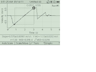
      First of all, we have to connect the GLX to the computer and capture the position and time graph. After we copied the graph on the word, we go to sub-menu and select 'Velocity' now we will see the graph of velocity versus time graph. We also have to copy down the graph on the word. Now, on the velocity graph, press right or left button to move the cursor to the point where cart start to move. Press F3 and select 'Linear Fit'. After recording the value of the slope, you deselect 'Linear Fit'. Open the axis menu and select 'acceleration'. Use left, right button to move cursor to the beginning of the experiment, and select 'Statistics' and measure the average value of acceleration.

Data table

Item	Value
Acceleration (slope)	0.570±0.00981 m/s^2
Acceleration (avg)	0.5 m/s^2

Graphs 

Acceleration versus time

Linear Fit Graph

Position graph

velocity graph

Conclusion

      Velocity was the instantaneous change of position and acceleration was the instantaneous change of velocity. Therefore, my hypothesis was correct since acceleration caused by gravity is constant as -9.81m*s^(-2), my velocity graph should be linear function and my position function should be parabola. However, since my GLX calculated to really useless decimal places, it had to be simplified by my hand. For this lab, I could not follow the instruction of the procedure and left out some graphs, so it would be better next time if i read through all instructions.

Questions.

   1. Describe the position versus time plot of the Graph screen. Why does the distance begin at a maximum and decrease as the cart moves up the inclined plane?

     the graph of the position function shows that the cart is moving back from a point, and it can be told that negative acceleration affected cart to convert velocity from positive to negative and therefor cart moves back.

   2. Describe the velocity versus time plot

     It changes it's sign, so it can be told that cart is moving to both direction

   3. Describe the acceleration versus time plot of the Graph display

     even though graph seems bumpy, it should be constant as -9.81

   4. How does the acceleration determined in the plot of velocity compare to the average value of acceleration from the plot of acceleration

     since we have to combine the secant lines of the velocity graph to determine acceleration, it is neither precise nor accurate. However, average value of acceleration is the sum of tangent line of velocity graph at all points, it is more precise and accurate.

Lap Report

Data

	D	F	H	M	P	10
Length (cm)	4.3	5.5	7	7.5	7.6	10.1
Width (cm)	3.6	3.6	3.9	7.4	7.6	8
Tickness(cm)	3.5	3.6	3.9	4.3	3.8	3.7
Mass (g)	27.62	38.8	51.2	96	161.1	177

Block	M	P	F	10	H	D
Time (s)	.78	.585	.725	.60	.56	.47
Distance (m)	1	1	1	1	1	1

Analysis
1. Organizing Data

	D	F	H	M	P	10
Volume (cm^3)	54.18	71.28	95.83	238.65	219.488	298.96

2. Analyzing Data
    a. 10.1-4.3
         =5.8
    b. 298.96-54.18
         =244.78
    c.  Multiplying several length measurements together to find the colume will make the data less procision because the number of the sigfig will decrease as we multiply numbers. As it is inferred in the data and a. and b., data don't show any ratio.
3. Analyzig Data
    No; because we didn't do this lab in complete vacuum condition, acceleration, resistace against air, and velosity of objects would be different.
4. Constructiong Graphs

Block	M	P	F	10	H	D
Time (s)	.78	.585	.725	.60	.56	.47
Distance (m)	1	1	1	1	1	1

Conclusions
5. Drawing Conclusions

D	F	H	M	P	10
27.62:53.18	38.8:71.28	51.2:95.83	96:238.65	161.1:219.488	177: 298.96

It can be inferred that ratio should be close to 1:2. but this data shows me that i have errors that changed my ratio. also it can be seen that if mass is increasing, than volume also increase except for block P
6. error can be maden when i measure the length, width, and depth. since human eyes are not maden to perfectly measure what is the length, quit few error can maden, and this will affect the data chart and volume. Moreover, when we were measuring the time for dropping blocks, there can also be few errors. First of all, our timer can show some error since we click the botton too fast or slow. secondly, since the area of the side that face the floor decide the resistance of air, there would be different measurement.

Extension
7. this experiment will show us about the timing that each students press the botton, and this explains the errors on the measuring the time